Homogeneous model optimization using grid search
In the previous tutorial, to introduce the basic functions of the toolbox, we ran a single simulation using some arbitrary model parameters. However, this simulation did not closely resemble the empirical functional imaging data of the HCP-YA train group, since we have not yet fit the model parameters to this empirical data.
There are several ways to fit the model parameters, ranging from simple brute-force approaches to more advanced optimization techniques. In this tutorial, we’ll focus on grid search, a straightforward method that involves systematically exploring a predefined range of parameter combinations. Grid search is only practical for low-dimensional parameter spaces, as the number of required simulations quickly explodes with increasing number of free parameters, due to the curse of dimensionality. Therefore, to keep things simple, here we will use a homogeneous rWW model, in which all brain regions share the same regional parameter values (\(w^{p}\), \(J^{N}\)). This is in contrast with the heterogeneous models, where regional parameters can vary across brain areas.
Running and saving the grid search
First, we’ll load the structural connectivity (SC) and target empirical BOLD data of the HCP-YA train group (pooled from the data of 706 subjects), which is the same as the data used in the first tutorial.
[1]:
from cubnm import datasets

# load structural connectome
sc = datasets.load_sc('strength', 'schaefer-100', 'group-train706')
# load empirical FC tril and FCD tril
emp_fc_tril = datasets.load_fc('schaefer-100', 'group-train706', exc_interhemispheric=True, return_tril=True)
emp_fcd_tril = datasets.load_fcd('schaefer-100', 'group-train706', exc_interhemispheric=True, return_tril=True)
Next, we define the simulation options, similar to the ones used in the first tutorial. However, we set states_ts=False to reduce GPU memory usage by the 1000 simulations of the grid search.
[2]:
sim_options = dict(
    duration=900,
    bold_remove_s=30,
    TR=0.72,
    sc=sc,
    sc_dist=None,
    dt='0.1',
    bw_dt='1.0',
    states_ts=False,
    states_sampling=None,
    noise_out=False,
    sim_seed=0,
    noise_segment_length=30,
    gof_terms=['+fc_corr', '-fcd_ks'],
    do_fc=True,
    do_fcd=True,
    window_size=30,
    window_step=5,
    fcd_drop_edges=True,
    exc_interhemispheric=True,
    bw_params='heinzle2016-3T',
    sim_verbose=True,
    do_fic=True,
    max_fic_trials=0,
    fic_penalty_scale=0.5,
)
We now define the optimization problem using BNMProblem.
[3]:
from cubnm import optimize

problem = optimize.BNMProblem(
    model = 'rWW',
    params = {
        'G': (0.001, 10.0),
        'w_p': (0, 2.0),
        'J_N': (0.001, 0.5)
    },
    emp_fc_tril = emp_fc_tril,
    emp_fcd_tril = emp_fcd_tril,
    out_dir = './grid',
    **sim_options
)
Here we specified the model (model), the free parameters to explore along with their ranges (params), and the empirical functional data we want to fit the simulations to (emp_fc_tril and emp_fcd_tril), and the simulation options defined above (**sim_options).
Note: When fitting the model to the data of an individual subject, instead of providing the emp_fc_tril and emp_fcd_tril it is possible to directly specify cleaned emp_bold. The empirical FC +/- FCD lower triangles will then be calculated based on the provided BOLD data.
We now create and run a grid search across all combinations of the free parameters defined in the BNMProblem. By sampling 10 points for each parameter ('G', 'w_p', 'J_N'), we end up running a total of 1000 (10^3) simulations.
The grid_shape argument of GridOptimizer.optimize() specifies how many values to sample for each parameter. These values are linearly spaced within the ranges defined earlier.
[4]:
# initialize the grid optimizer
grid = optimize.GridOptimizer()

# run the optimization on the `problem`
grid.optimize(problem, grid_shape={'G': 10, 'w_p': 10, 'J_N': 10})

# save the results in `out_dir`
grid.save()
WARNING:cubnm.sim.base:Progress cannot be shown in real time when using Jupyter, but simulations are running in background. Please wait...
Initializing GPU session...

CUDA device #0: NVIDIA A100-SXM4-40GB
Precalculating 60000000 noise elements...
noise will be repeated 30 times (nodes [rows] and timepoints [columns] will be shuffled in each repeat)
took 3.282247 s
Running 1000 simulations...
nodes: 100
N_SIMS: 1000
N_SCs: 1
BOLD_TR: 720
states_sampling: 720
time_steps: 900000
do_delay: 0
sim_seed: 0
exc_interhemispheric: 1
verbose: 1
progress_interval: 500
bold_remove_s: 30
drop_edges: 1
ext_out: 1
do_fc: 1
do_fcd: 1
states_ts: 0
noise_time_steps: 30000
100.00%
Simulations completed in 153.698605 s
Calculating simulated FC, dynamic FCs and FCD took 0.416841 s
Simulations and calculation of FC and FCD took 154.668668 s
Saving the optimal simulation
After running grid.optimize(), the simulated data can be accessed through grid.problem.sim_group. This includes the simulated BOLD signals, functional connectivity (FC) and functional connectivity dynamics (FCD) matrices, as well as state variables.
[5]:
print('BOLD shape:', grid.problem.sim_group.sim_bold.shape) # (sims, TRs, nodes)
print('FC trils shape:', grid.problem.sim_group.sim_fc_trils.shape) # (sims, edges)
print('FCD trils shape:', grid.problem.sim_group.sim_fcd_trils.shape) # (sims, window pairs)
print('State variables:', grid.problem.sim_group.sim_states.keys())
print('S_E shape:', grid.problem.sim_group.sim_states['S_E'].shape) # (sims, nodes); or (sims, time points, nodes) if `states_ts=True`
BOLD shape: (1000, 1250, 100)
FC trils shape: (1000, 2450)
FCD trils shape: (1000, 13861)
State variables: dict_keys(['I_E', 'I_I', 'r_E', 'r_I', 'S_E', 'S_I'])
S_E shape: (1000, 100)
In addition to the simulated data, the goodness-of-fit (GOF) to the empirical data and the cost function are calculated for each simulation and stored in grid.history. In this model, the cost function is calculated as cost = -(gof - fic_penalty), where gof = fc_corr - fc_diff - fcd_ks, and fic_penalty is a function of how much the time-averaged firing rates across nodes of each simulation diverge from 3 Hz.
The simulation with the lowest cost is selected as the optimal solution. The optimal parameters, along with their associated cost and goodness-of-fit components, are stored in grid.opt.
[6]:
grid.history.head()
The history saving thread hit an unexpected error (OperationalError('database is locked')).History will not be written to the database.
[6]:
| G | w_p | J_N | +fc_corr | -fcd_ks | +gof | -fic_penalty | cost | |
|---|---|---|---|---|---|---|---|---|
| 0 | 0.001 | 0.0 | 0.001000 | -0.032938 | -0.932017 | -0.964955 | 0.0 | 0.964955 |
| 1 | 0.001 | 0.0 | 0.056444 | -0.032612 | -0.932089 | -0.964701 | 0.0 | 0.964701 |
| 2 | 0.001 | 0.0 | 0.111889 | -0.032298 | -0.932089 | -0.964386 | 0.0 | 0.964386 |
| 3 | 0.001 | 0.0 | 0.167333 | -0.032015 | -0.932088 | -0.964103 | 0.0 | 0.964103 |
| 4 | 0.001 | 0.0 | 0.222778 | -0.031783 | -0.932158 | -0.963941 | 0.0 | 0.963941 |
[7]:
grid.opt
[7]:
G               1.112000
w_p             0.666667
J_N             0.389111
+fc_corr        0.303226
-fcd_ks        -0.144572
+gof            0.158653
-fic_penalty   -0.057502
cost           -0.101152
Name: 137, dtype: float64
Note: The evolutionary optimizers covered in the next tutorial behave similarly and have similar attributes, importantly including optimizer.history, optimizer.opt and optimizer.problem.sim_group.
When the optimizer results are saved by calling grid.save() method, the simulation and optimization configurations (including SC and target FC/FCD), optimizer history, averages of state variables (across time and nodes), and the optimal simulation parameters, its cost function components, as well as its simulated data are saved to disk.
[8]:
!ls -R ./grid/
./grid/:
grid_run-0

./grid/grid_run-0:
emp_fc_tril.txt   history.csv  opt_sim         problem.json  state_averages.csv
emp_fcd_tril.txt  opt.csv      optimizer.json  sc.txt

./grid/grid_run-0/opt_sim:
sim_data.npz
All output files are stored in the specified out_dir (here: './grid/'), within a subdirectory named using the format <optimizer_name>_run-<run_idx>, e.g., 'grid_run-0'. The optimizer name is based on the optimizer class (e.g. GridOptimizer -> 'grid'), and the run index is assigned automatically to prevent overwriting the results of previous optimization runs.
Contents of each run directory are:
'emp_bold.txt','emp_fc_tril.txt','emp_fcd_tril.txt','sc.txt'(and'sc_dist'in simulations with conduction delay): The input arrays. Note that here we only had provided the empirical BOLD, and empirical FC and FCD were calculated from it.'history.csv': Contains the history of all simulations run by the optimizer, including the sampled free parameters and their associated evaluation metrics (goodness-of-fit, cost, and their components). Additionally,'opt_history.csv'is created for evolutionary optimizers but not for the grid search.'opt.csv': Contains the free parameters and evaluation metrics of the optimal simulation (or simulations, when using multi-objective optimizers).'opt_sim/sim_data.npz': Compressed NumPy archive containing the simulated data and parameters of the optimal simulation(s).'state_averages.csv': Averages of model state variables (across time and nodes) for each simulation (Only saved when using theGridOptimizer).'problem.json': JSON-serialized configuration of theBNMProblem.'optimizer.json': JSON-serialized configuration of the optimization run.
Visualization of the grid
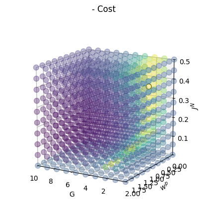
To show how the model behaves across different parameter combinations, we can visualize how the cost function, goodness-of-fit, and its components (FC correlation, FC absolute mean difference, FCD KS distance, and FIC penalty) vary as functions of the model’s free parameters: 'G', 'w_p', and 'J_N'.
We will first visualize the cost function. Here, to indicate better simulations with higher values, rather than the cost function we will visualize negative cost function. In this and the subsequent parameter space plots, the optimal simulation (with lowest cost, or highest negative cost) is shown with a black outline.
[9]:
import matplotlib.pyplot as plt

grid.plot_space('-cost', opt=True, config=dict(size=60, alpha=0.35, azim=120))
plt.tight_layout()
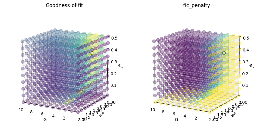
In this model, cost function is calculated as - (gof - fic_penalty). We can next visualize these components of cost function, which are included in +gof and -fic_penalty columns of cmaes.history.
The signs in front of each cost component indicate the optimization direction: a + sign means the quantity is maximized, while a - sign means it is minimized.
For example: +gof (maximize goodness-of-fit), +fc_corr (maximize FC correlation), -fcd_ks (minimize FCD KS distance), -fic_penalty (minimize FIC penalty).
Note: FIC penalty in rWW model can be disabled by setting fic_penalty_scale = 0 when creating the BNMProblem object.
[10]:
fig, axes = plt.subplots(1, 2, figsize=(9, 4.5), subplot_kw={'projection': '3d'})
for i, var in enumerate(['+gof', '-fic_penalty']):
    grid.plot_space(var, opt=True, config=dict(size=60, alpha=0.35, azim=120), ax=axes[i])
fig.tight_layout()
The goodness-of-fit (+gof) itself is composed of two components: +gof = (+fc_corr) + (-fcd_ks). Next, we will visualize these components:
[11]:
fig, axes = plt.subplots(1, 2, figsize=(9, 4.5), subplot_kw={'projection': '3d'})
for i, var in enumerate(['+fc_corr', '-fcd_ks']):
    grid.plot_space(var, opt=True, config=dict(size=60, alpha=0.35, azim=120), ax=axes[i])
fig.tight_layout()
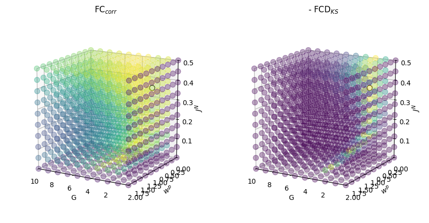
The plots above show that while many parameter combinations result in high FC correlation and low FIC penalty (i.e., higher values of +fc_corr and -fic_penalty), only a narrow band of parameter values leads to simulations with realistic dynamics, as reflected by higher values of -fcd_ks. This pattern is in turn reflected in the grids of +gof and negative cost.
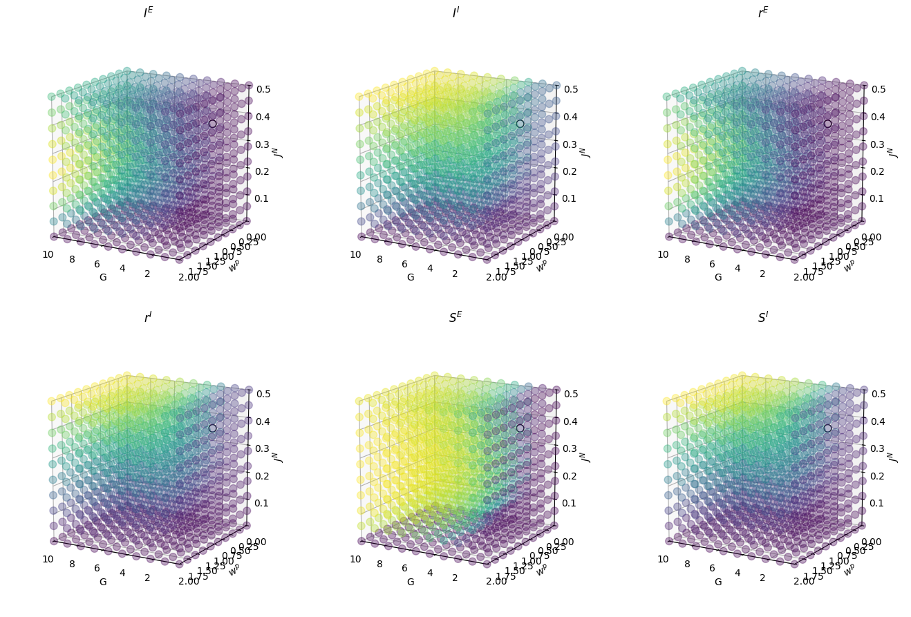
In addition to the evaluation metrics plotted above, we can also visualize how average state variables vary across the parameter space. This can provide further insights into how the model’s behavior changes as a function of different parameters.
[12]:
fig, axes = plt.subplots(2, 3, figsize=(13.5, 9), subplot_kw={'projection': '3d'})
axes = axes.flatten()
for i, var in enumerate(grid.problem.sim_group.sim_states.keys()):
    grid.plot_space(var, opt=True, config=dict(size=60, alpha=0.35, azim=120), ax=axes[i])
fig.tight_layout()
Visualization of the optimal simulation
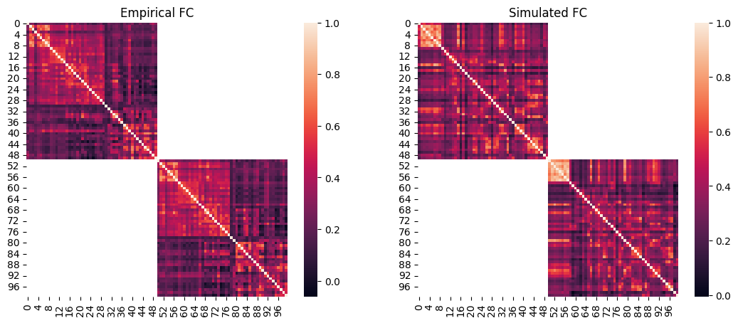
Lastly, we will visualize the simulated FC and FCD of the optimal simulation and compare them to the empirical data.
We can then plot the empirical group-averaged FC next to the simulated FC:
[13]:
import seaborn as sns

# load the squared form of the empirical FC
emp_fc = datasets.load_fc('schaefer-100', 'group-train706', exc_interhemispheric=True, return_tril=False)


# determine the index of optimal simulation
# which is the name of the optimum pandas Series
opt_idx = grid.opt.name

# load squared form of optimal simulated FC
sim_fc = grid.problem.sim_group.get_sim_fc(opt_idx)

# plot it next to the empirical FC
fig, axes = plt.subplots(1, 2, figsize=(13, 5))
sns.heatmap(emp_fc, ax=axes[0])
axes[0].set_title("Empirical FC")
sns.heatmap(sim_fc, ax=axes[1])
axes[1].set_title("Simulated FC")
[13]:
Text(0.5, 1.0, 'Simulated FC')
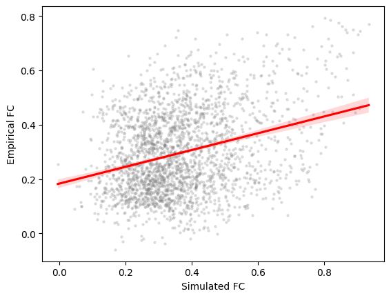
[14]:
import scipy.stats

# regression plot
fig, ax = plt.subplots()
sns.regplot(
    x=grid.problem.sim_group.sim_fc_trils[opt_idx],
    y=emp_fc_tril,
    scatter_kws=dict(s=5, alpha=0.2, color="grey"),
    line_kws=dict(color="red"),
)
ax.set_xlabel("Simulated FC")
ax.set_ylabel("Empirical FC")

# calculate Pearson correlation
print(f"FC correlation = {scipy.stats.pearsonr(grid.problem.sim_group.sim_fc_trils[opt_idx], emp_fc_tril).statistic}")
FC correlation = 0.30322564112211214
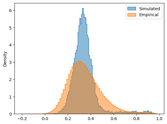
In addition to static FC, we can also plot the simulated FCD matrix distribution next to the empirical FCD (pooled across the group), and calculate their Kolmogorov-Smirnov distance:
[15]:
# plot the distributions next to each other
sns.histplot(grid.problem.sim_group.sim_fcd_trils[opt_idx], element='step', alpha=0.5, label='Simulated', stat='density')
ax = sns.histplot(emp_fcd_tril, element='step', alpha=0.5, label='Empirical', stat='density')
ax.legend()

# calculate KS distance
print(f"FCD KS distance = {scipy.stats.ks_2samp(emp_fcd_tril, grid.problem.sim_group.sim_fcd_trils[opt_idx]).statistic}")
FCD KS distance = 0.14457225238790572
The fit of simulated FC and FCD to the empirical data is quantified as +fc_corr and -fcd_ks, which are combined to define +gof. These evaluation metrics as well as the optimal parameters are stored in grid.opt:
[16]:
grid.opt
[16]:
G               1.112000
w_p             0.666667
J_N             0.389111
+fc_corr        0.303226
-fcd_ks        -0.144572
+gof            0.158653
-fic_penalty   -0.057502
cost           -0.101152
Name: 137, dtype: float64
We observe that, after tuning model parameters using grid search, the simulated FC and FCD more closely resemble the empirical FC and FCD compared to the simulation performed with arbitrary parameters in the previous tutorial.
However, as we will explore in the next tutorials, there is still room for improvement, in terms of both the optimization approach and the model.